QTL analysis plugins

All QGene's QTL, marker, and trait-analysis methods are written as plugins. A plugin is a relatively small piece of program code meant to be "plugged in" to a larger program that finds it after the larger program is started by the user. If you are a developer, you already know this. If you aren't, it's all you need to know.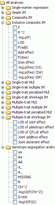

The purpose of this page is to describe each of the plugin analyses we've provided. Others will be described as they are contributed.

Should you use all of them in analyzing your data set? Certainly not. They are presented only for comparison with one another. I personally (CN) rarely use any QGene mapping methods but single- or multiple-trait MIM. We've implemented a couple of undocumented methods whose advantages, if any, haven't been well investigated, and don't expect anyone to trust them until they have.

Plugins for the QTL analysis window

All of these are for QTL analysis except for the Genotype segregation analysis plugin, which was added to this window because it generates contours drawn on the genetic map.

For each plugin a variety of statistics may be computed, drawn, and exported as a tabular text file. To see and select these statistics, open up the stats list for the plugin by clicking on the hinge icon at left of its label. P-value statistics are shown as -1 times their log to base 10; for example -log10(P(Chi^2)) for segregation stats. If you choose a signed effect statistic such as Add effect (additive effect), you will want to know how the sign corresponds to the parent whose allele increases the phenotypic value. This is labeled on the effect plot as follows: a positive-signed effect represents an increasing allele from parent 1, the A parent; a negative-signed effect, an increasing allele from parent 2, the B parent.

Single-marker regression

The simplest method of QTL finding, this regresses phenotypic on marker-genotype values, which may be represented as 0, 1, and 2, or -1, 0, and 1, for genotypes aa, Aa, and AA respectively. But what is done with missing data or dominant markers (the latter represented by genotype values A_ and a_)? Individuals lacking phenotype data are dropped. Missing or incompletely informative markers are replaced with their expectations based on flanking markers, via the algorithm of Jiang & Zeng (1997). This makes QGene's SMR useless unless a genetic map is available. Even then it's provided only for comparison, not for serious QTL mapping!

Simple interval mapping (SIM)

Regression on the expectation of genotype at each tested QTL position on the map, by the method of Haley & Knott (1992). Like all of QGene's interval methods, QGene's SIM performs QTL tests every 2 cM by default, but this setting can be changed globally in the main QGene Options menu.

Composite IM (CIM-LS)

Implementation of the least-squares method of Zeng (1994). At present the cofactor-dropping window is fixed at 15 cM. If no cofactors are selected, this is the same as SIM.

Inclusive composite IM (ICIM)

Implementation of the method of Li et al. (2007). We don't see any advantages to this method over regular CIM in speed or accuracy, but you can investigate for yourself.

Single-trait MLE (CIM-MLE)

If no cofactors are selected, this is the same as the method of Lander & Botstein (1989).

Single-trait multiple IM (MIM)

Implementation of the method of Kao & Zeng (1999).

Single-trait penalized MLE (PMLE)

Implementation of the method of Xu (2003).

Single-trait shrinkage IM (ShrinkIM)

Implementation of an as-yet unpublished method of Z. Guo & R. Joehanes.

Bayesian interval mapping (BIM)

QGene's BIM is based on methods of Sillanpää and Arjas (1998), with these differences:

• The QTL death step is done after the QTL-move and QTL-effect-update steps.
• The scan is done by steps of 2 cM (adjustable), instead of by marker interval.
• Algorithmic optimization, such as extensions of QR decomposition, is used to minimize execution time.
• No smoothing is applied.

What is plotted in the upper profile above is the proportion of reversible-jump-Markov-chain Monte Carlo (RJ-MCMC) iterations (cycles) in which each QTL position has been visited. In the lower profile is plotted the value of the additive effect, averaged over the visits to each position. In mating designs allowing dominance estimation, this effect too can be plotted.

Bayesian interval mapping, though attractive for its power to explore QTL model space, is hard for the average QTL mapper to understand, no one really knows yet whether it produces results superior to those of MIM or other mapping methods, there is no reliable way to assign significance thresholds, and the amount of computing required makes investigating these questions hard. Even with optimizations that make BIM faster in QGene than in other QTL software, a population of size 300 with a map of 1200 cM may require, depending on your computer's speed, several minutes to half an hour for each trait. BIM computation will hog CPU cycles and tie up your machine. If you have many traits, you may like to select them before choosing BIM, and let the program run overnight. But be aware that QGene uses around 15 Mb of memory to store the results of BIM for each trait, and unless your machine has a Gb or more of free memory, it may run out. In this case you'll see an "Out of memory" error in the error log, and are best advised to close the program and start over.

(QTL mappers don't often report having used Bayesian interval mapping for real data...)

After you have either completed or canceled a BIM run, the profile based on the completed MCMC cycles will appear in the analysis window. Now, whenever the trait for which you have run BIM is selected in the trait list, you may choose Options/Single-trait Bayesian IM from the QTL-analysis window's menu bar,

bringing up the following dialog:

The plots show the parameter values visited during the MCMC cycles computed by QGene. QGene's default is 60,000 cycles, preceded by 600 burn-in cycles and thinned to one cycle in each 20. Entering new values for burn-in time and thinning interval will change these plots (and the QTL profile in the analysis window) as soon as you press the Tab key to leave the corresponding text box, or click with the mouse in a different text box. You may also add any number of MCMC cycles without starting over: just type a value in the Cycles from current state box, and press the Go button. Be aware that in this case you won't get a progress dialog allowing you to cancel the run -- so avoid entering many thousands of cycles if you don't want to wait!

Multiple-trait MLE (MT-MLE)

Implementation of the method of Jiang & Zeng (1995).

Multiple-trait multiple IM (MT-MIM)

Implementation by R. Joehanes of an unpublished multiple-trait adaptation of MIM.

Multiple-trait penalized MLE (MT-PMLE)

Implementation by R. Joehanes of an unpublished multiple-trait adaptation of PMLE..

Multiple-trait shrinkage IM (MT-ShrinkIM)

Implementation by R. Joehanes of the multiple-trait adaptation of ShrinkIM.

MLE-GLZ and MIM-GLZ

These two GLZ plugins are based on the Generalized Linear Model (GLZ) and intended for mapping QTLs in non-normally distributed trait data. They will output only LOD scores, not QTL effects. The details will be described in an article currently in preparation. Both plugins check the trait data and attempt to apply an appropriate analysis, using these distributions and link functions for these trait types:

• binary (either nominal or ordinal): binomial distribution with logit link
• nominal with > 2 categories: multinomial distribution with multinomial logit link.
• ordinal with > 2 categories: multinomial distribution with cumulative logit link
• metric, nonnegative integer: negative binomial distribution with log link (the data are treated as count data)
• otherwise (metric, not count data): normal distribution with identity link. In this case, the MLE-GLZ will fall back to MLE and MIM-GLZ will fall back to MIM. The results of MLE-GLZ and MLE, and MIM-GLZ and MIM will be the same except for rounding errors.
  

The link functions and distributions provided by QGene may be selected in the Options menu of your main QTL window. You can map QTLs in survival or censored data, for example.

With non-normal data, you must use permutation testing to determine the significance threshold. Don't expect the LOD score (which we might better call a pseudo-LOD score, for reasons described in a more technical presentation elsewhere) to approach conventional thresholds. It can be very low (< 1) and still highly significant by permutation test.

Genotype segregation analysis

While this isn't a QTL-analysis method, it was convenient to place it with other methods that yield plots of statistics along chromosomes. The various phenotype labels show the proportion of the population that carry the indicated allele at every map position. To use the feature, you must select a trait in the trait list at left -- even though the analysis makes no use of trait data. Note that by selecting the genotype classes of interest, N, and a desired statistic and then using the File menu to export the results to a file or to the Clipboard, you will get a useful segregation table for convenient viewing in a spreadsheet program.

Generalized R²

Most of QGene's QTL methods generate likelihood (LOD) rather than regression statistics. Because many analysts using CIM or MIM wish to report an estimate of the explanatory power of a QTL, QGene offers a "generalized" R² derived from Nagelkerke (1991) as
R² = 1 - 10^{(-2 LOD / n)}
where n is the number of observations (in the commonest QTL model, the population size).

References

1. Haley, C.S. & S.A. Knott. 1992. A simple regression method for mapping quantitative trait loci in line crosses using flanking markers. Heredity 69:315-324.
2. Jiang, C. & Z.-B. Zeng. 1995. Multiple trait analysis of genetic mapping for quantitative trait loci. Genetics 140:1111-1127.
3. Jiang, C. & Z.-B. Zeng. 1997. Mapping quantitative trait loci with dominant and missing markers in various crosses from two inbred lines. Genetica 101:47-58.
4. Kao, C.-H. & Z.-B. Zeng. 1999. Multiple interval mapping for quantitative trait loci. Genetics 152:1203-1216.
5. Lander, E.S. & D. Botstein. 1989. Mapping Mendelian factors underlying quantitative traits using RFLP linkage maps. Genetics 121:185-199.
6. Li, H., G. Ye & J. Wang. 2007. A modified algorithm for the improvement of composite interval mapping. Genetics 175:361-374.
7. Sillanpää, M. J. & E. Arjas. 1998. Bayesian mapping of multiple quantitative trait loci from incomplete inbred line cross data. Genetics 148: 1373-1388
8. Xu, S., 2003  Estimating polygenic effects using markers of the entire genome. Genetics 163:789-801.
9. Zeng, Z.-B. 1994. Precision mapping of quantitative trait loci. Genetics 136:1457-1468.
10. Nagelkerke, N. J. D. 1991 A note on a general definition of the
    coefficient of determination. Biometrika 78(3): 691-692.